We often like to know something about the entire population; however, due to time, cost, and other restrictions, we can only take a sample of the target population. The idea of a sample (as discussed in Chapter 1) is an exploration from the part to the whole. In order to take a sample, it must be chosen carefully by following established procedures and distributions. The idea behind the population distribution is that it is derived from the information on all elements of the population being studied. In comparison, a sampling distribution consists of a random sample that represents the entire population. There are many types of sampling methodologies, but the five most common include: Random sampling, Systematic sampling, Convenience sampling, Cluster sampling, and Stratified sampling. In Chapter 7, we discussed selecting a random variable, where we illustrated how to find a simple random variable by using a sample command:

Simple Random sampling in R:

>x <- 1:10 # Your dataset from 1 to 10
>sample(x) # Your sample
[1] 3 2 1 10 7 9 4 8 6 5
sample(10) # asking R to generate 10 numbers.
[1] 10 7 4 8 2 6 1 9 5 3

However, there are other methodologies for sampling including systematic sampling, cluster sampling and stratified  sampling.

Systematic sampling command in R:

# population of size N
# the values of N and n must be provided
>sys.sample = function(N,n){
>k = ceiling(N/n)
#ceiling(x) rounds to the nearest integer that’s larger than x.
#This means ceiling (2.1) = 3
>r = sample(1:k, 1)
>sys.samp = seq(r, r + k*(n-1), k)
>cat(“The selected systematic sample is: \””, sys.samp, “\”\n”)
#Note: the last command “\”\n” prints the result in a
}
#To select a systematic sample, we will use the values of N and n
in the following command:
>sys.sample(50, 5)

Convenience sampling in R:

R does not support convenience sampling. Researchers can use utilities in R to summarize the data collected from convenience sampling.

Cluster sampling in R:

A cluster sample is a probability sample in which each sampling unit is a collection or a group of elements. It is useful when a list of elements of the population is not available but it is easy to obtain a list of clusters.
In R:
>cluster.mu <- function(N, m.vec, y, total=T, M=NA) {
# N = number of clusters in population
# M = number of elements in the population
# m.vec = vector of the cluster sizes in the sample
# y = either a vector of totals per cluster, or a list of
# the observations per cluster (this is set by total)
>n <- length(m.vec)
# If M is unknown, m.bar is estimated with the mean of m.vec
>if(is.na(M)) {mbar <- mean(m.vec)}
>else {mbar <- M/N}
# If there are not totals of observations they are computed
>if(total==F) {y <- unlist(lapply(y,sum))}
>mu.hat <- sum(y)/sum(m.vec)
>s2.c <- sum((y-(mu.hat*m.vec))ˆ2)/(n-1)
>var.mu.hat <- ((N-n)/(N*n*mbarˆ2))*s2.c
>B <- 2*sqrt(var.mu.hat)
>cbind(mu.hat,s2.c,var.mu.hat,B)
}

Stratified sampling:

This type of sampling is based on  a population sample that requires the population to be divided into smaller groups, called ‘strata’. Random samples can be taken from each stratum, or group. 
In R there is a function called stratified_sampling. The code for it includes:
>stratified_sampling<-function(df,id, size) {
#df is the data to sample from
#id is the column to use for the groups to sample
#size is the count you want to sample from each group
# Order the data based on the groups
>df<-df[order(df[,id],decreasing = FALSE),]
# Get unique groups
groups<-unique(df[,id])
group.counts<-c(0,table(df[,id]))
#group.counts<-table(df[,id])
>rows<-mat.or.vec(nr=size, nc=length(groups))
# Generate a matrix of sample rows for each group
#for (i in 1:(length(group.counts)-1)) {
>start.row<-sum(group.countsi])+1
>samp<-sample(group.counts[i+1]-1,size,replace=FALSE)
>rows[,i]<-start.row+samp
}
>sample.rows<-as.vector(rows df[sample.rows,]
}

Sampling Distribution

The sampling distribution of a particular statistic is the distribution of all possible values of the statistic, computed from samples of the same size randomly drawn from the same population. In order to conduct a successful sampling distribution, we need to provide an equal chance of selection for all units found in the entire population. The calculation of the sampling distribution needs to be an estimation of the entire population distribution versus the sample distribution.

The concept behind a sampling distribution is the probability distribution of a sample given a finite population with mean (μ) and variance (σ2). The calculation of the sampling distribution needs to be an estimation of the entire population distribution versus the sample distribution. As a result, we need to compare the population values also known as parameters to sample values also known as statistics. What happens if we do not have the information about the value of x? The Central Limit Theorem tell us what we should expect.

The Central Limit Theorem

The Central Limit Theorem states that the distribution of the sum (or average) of a large number of independent, identically distributed variables will be approximately normal, regardless of the underlying distribution. The importance of the Central Limit Theorem is hard to overstate; indeed it is the reason that many statistical procedures work. For any distribution with finite mean and standard deviation, samples taken from that population will tend towards a normal distribution around the mean of the population as sample size increases. Furthermore, as sample size increases, the variation of the sample means will decrease.

The formulas of the Central Limit Theorem:

 

 

 

 

 

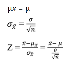
Where:
n = sample size
x = number of success

In order to calculate the three formulas above, we follow 5 common steps to finalize our result. 
Step 1: Calculate the following values:
The mean (average or μ), the standard deviation (σ), the population size, sample size (n), and the number associated with “greater than” is represented by .
Step 2:  Draw a graph that identifies the mean.
Step 3: Find the z-score using the second formula by:
3.1: Subtracting the mean (μ in step 1) from the ‘greater than’ value (in step 1).
3.2: Dividing the standard deviation (σ in step 1) by the square root of your sample (n in step 1).
3.3:  And last, divide your result from step 1 by your result from step 2 (i.e. step 1/step 2)
Step 4:  Find out the z-score you calculated in step 3.
Step 5: Convert the decimal in step 4 to a percentage.

In order to employ R, we will use the rnorm command to draw 500 numbers at random distribution. The mean for this distribution is 100 and standard deviation is 10.

>x =rnorm (500, mean=100, sd=10)
>x

[1] 111	55209 97	24050 92	68848 82	52463 109	31802 108	32459 83	00670 89	26875
[9] 75	70270 123	58992 102	09190 119	77364 88	12079 106	97782 98	59419 103	14760
[17] 94	61791 88	13449 99	29828 91	85665 104	26802 94	80050 108	50890 84	33962
[25] 101	09177 81	12858 91	36644 96	93328 99	12372 112	96364 107	81306 107	95731
[33] 96	43726 108	51994 109	68077 104	83131 99	32821 103	60105 104	19988 93	96107
[41] 102	33610 93	78330 124	02103 94	78894 105	64514 95	79113 104	30137 89	44551
[49] 113	75918 93	31709 117	63567 107	31241 128	34292 112	88165 107	20717 113	37049
[57] 100	59420 113	03992 115	58488 88	73811 72	85903 105	96066 107	92803 103	03057
[65] 104	83090 105	81510 87	53651 94	72101 111	60492 107	54120 91	60892 90	55675
[73] 93	22649 101	25328 107	63417 102	67403 81	29807 83	06487 93	36482 93	70351
[81] 108	06343 107	03462 95	92501 93	33976 109	85680 91	24292 105	56427 90	46225
[89] 96	69797 99	28140 99	63375 91	76809 94	70627 96	59201 95	13531 117	79783
[97] 92	33372 86	74711 88	56511 102	06469 119	70357 104	40460 102	09666 101	34539
[105] 103	59292 99	32866 101	01474 101	58607 93	74571 108	59612 100	67548 116	78889
[113] 96	80618 92	62621 107	17173 96	38856 100	68643 110	06115 112	36466 105	30423
[121] 92	38832 100	10897 97	82776 111	70773 88	82512 95	20199 114	80327 97	45863
[129] 107	50334 98	10763 102	99769 106	39846 99	29961 93	20238 93	00196 100	03094
[137] 113	50025 115	03300 106	32779 89	58524 85	14172 103	70424 100	34439 108	09727
[145] 79	72313 96	22978 109	05198 101	18664 126	50670 98	57598 92	38971 99	55717
[153] 103	14452 109	05158 100	54290 112	65490 106	79928 107	35994 90	53019 81	14386
[161] 98	61420 107	48035 103	12688 87	12294 99	08614 92	89029 105	88213 82	92831
[169] 96	59139 105	29636 87	87654 105	41993 89	64116 101	23920 103	23246 114	41911
[177] 90	83871 94	73443 122	92020 105	40389 113	58954 117	54110 97	64189 89	95689
[185] 93	08089 88	92455 87	16113 84	23658 95	56815 95	85473 87	22373 105	84172
[193] 92	83464 120	95720 83	94792 107	77612 103	19188 95	49539 108	04202 96	85295
[201] 84	46574 105	08998 83	23930 97	22247 102	00901 92	78544 86	53811 104	21367
[209] 97	33453 85	86610 108	69772 132	01008 97	67792 103	33140 106	23286 111	31900
[217] 102	36186 100	79340 108	32016 102	86359 88	64807 107	88597 82	06701 110	22867
[225] 100	56341 116	09703 101	08097 90	05288 105	50572 106	99322 87	18559 106	81418
[233] 86	26361 95	58739 81	64357 80	85432 95	59627 96	56567 106	28033 96	22533
[241] 122	20326 99	91373 100	35222 106	86913 89	19629 93	93497 101	01534 106	37162
[249] 87	15815 123	24625 104	89270 111	01097 90	56193 105	84058 79	86703 93	41226
[257] 93	70946 106	57830 92	83771 108	41502 102	25140 92	66213 102	31731 99	12675
[265] 119	67439 93	27267 83	21695 110	74516 99	94568 107	07684 84	85125 96	75518
[273] 112	35921 84	27979 90	43687 112	41555 103	83653 93	43820 112	05262 102	78605
[281] 103	96401 106	47644 86	41875 103	98403 112	21884 91	61851 103	52600 99	98722
[289] 105	73103 106	45804 73	32174 113	81926 86	30343 111	53781 94	86229 86	85868
[297] 110	95911 93	40308 99	60810 111	86818 93	71954 88	57434 98	63304 94	37386
[305] 100	48269 100	69264 86	07424 105	78913 83	79600 94	39545 95	09701 88	31949
[313] 102	05952 94	12686 91	06158 84	04382 95	39729 91	38391 96	83824 101	20211
[321] 89	17918 121	25700 122	52074 94	68952 97	63818 119	14110 92	14390 91	88988
[329] 113	75349 91	35794 74	76374 105	51984 111	06501 84	27096 86	24828 102	40973
[337] 104	25186 97	94886 109	30634 92	43647 99	71722 95	93561 85	92015 85	50492
[345] 107	81461 106	31641 104	20502 88	97319 100	24124 95	01394 104	78500 103	32714
[353] 104	20762 91	42431 99	56947 102	71849 95	55139 93	43830 92	29035 86	74374
[361] 102	31213 99	86325 80	84533 97	25405 108	02706 100	67164 104	06942 104	42769
[369] 95	64327 109	67884 92	69703 114	91947 82	97577 95	49521 124	46985 104	86343
[377] 96	00504 100	57825 104	14272 98	45316 114	32171 95	36987 82	69245 86	88861
[385] 101	88278 107	88787 110	60463 96	09254 106	85077 116	36704 103	05464 79	10533
[393] 106	07226 95	35260 95	05443 82	31125 91	84258 87	62534 106	14509 100	58569
[401] 85	90184 100	76999 102	43461 109	64790 96	92951 100	46193 90	81334 81	38203
[409] 106	13624 104	94034 93	40309 90	61116 97	41716 109	74482 85	08824 120	28829
[417] 94	94676 109	19260 112	24533 98	41927 97	95787 100	95752 102	60309 101	35629
[425] 109	01787 95	92091 110	40156 108	74196 102	84021 109	40487 101	92498 104	08255
[433] 98	13174 106	96881 89	61117 93	13745 114	03345 108	75272 107	21131 93	17538
[441] 103	96577 81	18744 120	59262 103	66089 112	42153 100	22605 97	28623 102	52154
[449] 80	32988 90	94998 83	25729 92	70170 105	04413 112	67451 91	90482 99	54297
[457] 95	13043 117	91574 102	77992 97	96377 91	23315 105	69915 102	54660 66	25475
[465] 84	98554 102	48492 110	85954 84	19404 108	13689 109	41963 91	33799 113	34345
[473] 86	90366 96	23221 111	91153 98	64547 83	28638 102	55118 97	14488 118	38495
[481] 95	12027 97	51625 94	63760 105	75733 103	73914 105	37714 112	00177 120	35917
[489] 104	20671 89	17663 100	23328 99	87450 116	70476 86	93272 110	40801 102	18216
[497] 100	51997 82	10726 105	22389 105	46758

When you examine the numbers stored in R generated for x, it is hard to see if the mean of this distribution is equal to 100 as we asked. In order to overcome this perception, we will employ the histogram function to see the visual distribution of 500 random variables.

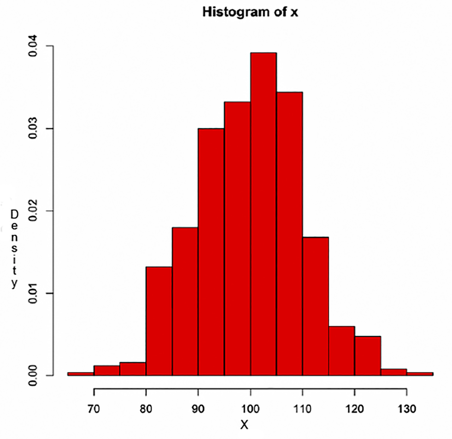
Using just the population mean [μ = 99.86607] and standard deviation [σ = 10.17966], we can calculate the z-score for any given value of x. In this example, we will use the value of variance equals 103.6256

>z <– (103.6256 – 99.83306) / 10.17966
>z
[1] 0.3725606
Find the value on the z-score table.
The score is converted to a percentage and it is equal to 37.25%.

Next, Chapter 10, Confidence Interval Estimation
Previous, Chapter 8, Random Variables and Probability