
The subject of random variables plays an important part in any probability distributions. The term random variable is often associated with the idea that value is subject to variations due to chance. We often encounter random variables in library science literature with two specific outcomes: discrete distribution and binomial distribution.
In R, to generate a random integer between 1 and 40 , we use the sample function:
>sample(1:40,4)
[1] 2 21 6 9
Another way to generate a random number is using the runif function. This function will allow us to select a number between minimum and maximum that is equally likely to occur.
>x1 <- runif(1, 5.0, 7.5)
>x1
[1] 6.715697
In this function, it allows us to generate one random integer between 5.0 and 7.5.
A Discrete Distribution is a random variable defined as a countable variable. To illustrate this type of distribution, let’s take the number of copies of Dostoyevsky’s Humiliated and Insulted found in the library. This number will not change as long as the library keeps track of these copies.
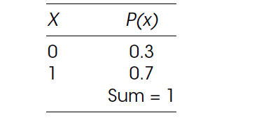
In order to illustrate discrete distributions, we will use the Bernoulli distribution. Bernoulli was known for his work on probability statistics and was one of the founders of the calculus of variations. Under this distribution there are only two possible values of the random variable, x = 0 or x = 1. When drawing numbers from this distribution, if selecting x = 0, the probability is P(x) = 0.3, while the probability of selecting x = 1 is 0.7.
However, we still need to find out the Mean and Standard Distribution in order to fully evaluate its values. The mean of a discrete variable is denoted by μ (mu). It is the actual mean of its probability. It is also called the expected value and is denoted by E(x). The mean or expected value of a discrete variable is the value that we expect to observe per repetition of the experiment we conduct over a large number of times.
To calculate the mean of a discrete random variable x, we multiply each value of x by the corresponding probability and sum (hence the symbol, Σ). This sum gives us the mean (or expected value) of the discrete random variable x. The formula for the expected discrete random variable is: μ = ΣxP(x)
In R, we use the table above for the two variables x and p. To calculate the mean, we need to multiply the corresponding values of x and p and add them. We will call the result of this calculation mu.
>x <– c(0,1)
>p <–c(0.3, 0.7)
>mu <- sum(x * p)
>mu
[1] 0.7
The result 0.7 is the value of the mean.
The Standard Deviation of a discrete random variable is denoted by σ (sigma) and measures the spread of the probability distribution. A higher level for the standard deviation of a discrete random variable indicates that x can assume values over a larger range from the mean. In contrast, a smaller value for the standard deviation indicates that most of the values that x can assume are clustered closely to the mean. The formula for the standard deviation of a discrete random variable consists of:
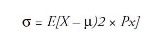
In order to use R to calculate the value of σ square, we subtract the value of mu from each entry in x, square the answers, multiply by p, to reach the sum.
>sigma2 <- sum((x-mu)^2 * p)
>sigma
[1] -2.17
The second form of discrete probability distribution is Binomial Distribution. It describes the behavior of a count variable x if the following conditions apply:
1: The number of observations n is fixed.
2: Each observation is independent.
3: Each observation represents one of two outcomes (“success” or “failure”).
4: The probability of “success” p is the same for each outcome
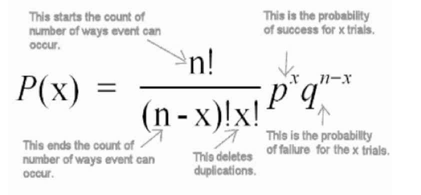 where P(x) = Probability of x success given the parameters n and p
n = sample size
p = probability of success
1 – p = probability of failure
x = number of successes in the sample (x = 0,1,2,3,4……n)
The binomial distribution in R is noted as dbinom. There are three required arguments for binomial calculation: the value(s) for which to compute the probability (k), the number of trials (n), and the success probability for each trial (θ). In the previous example, we employed all three values that include: 2 as the probability value of k, 2 is the number of trials , and 0.7 for success probability for each trial.
>dbinom(2, 2, 0.7)
where (x = 2, size = 2, prob = 0.7)
[1] 0.49
In R, the argument is pursued in the following manner:
x, q = vectors of quartiles
P = vector of probabilities
n = number of observations. If length (n) > 1, the length is taken to be the number required.
size = number of trials
In the textbook you will find more details on the Characteristics of Binomial Distribution and Normal Distribution.
Next, Chapter 9, Sampling Distributions
Previous, Chapter 7, Probability Theory