When we conduct research with only two central variables, these variables become the theme of our research methodology. In order to analyze the correlation between two variables, we consult bivariate statistics to search out the embedded information. The term correlation is often associated with the terms association, relationship, and causation.

We will only look at the Pearson sample correlation coefficient and its properties.

Pearson sample correlation coefficient measures the strength of any linear relationship between two numerical variables. A Pearson sample correlation coefficient attempts to draw a line of best fit through the data points of two variables. The Pearson sample correlation coefficient, r, indicates how far away all these data points are to this line of best fit, i.e., how well the data points fit this new model/line of best fit. Its value can range from -1 for a perfect negative linear relationship to +1 for a perfect positive linear relationship. A value of 0 (zero) indicates no relationship between the two variables.

The Pearson sample correlation coefficient formula: 

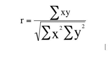
r = [Equation]
Σ = Number of pairs of sources
Σxy = Sum of the products of paired scores
Σx = Sum of x scores
Σy = Sum of y scores
Σx2 = Sum of squared x scores
Σy2 = Sum of squared y scores

In order to practice the Pearson sample correlation coefficient formula between two variables x and y, we will employ the data presented in the table below. In this table, the value x refers to the number of visitors to the special collections room in the library.  y stands for the number of visitors to the old newspaper archive collection room. Our objective is to compute the similarity between these two variables. The data for the two rooms used in our library research:

X	Y
Visitors to special collections room	Visitors to old newspaper archive collections room
1	4
3	6
5	10
5	12
6	13

To download the file, click Table 6.1

Using Pearson sample correlation coefficient can show the correlation between the number of visitors to the special collections room and the number of visitors to both rooms. To achieve this value, Pearson sample correlation coefficient is computed by dividing the sum of the xy column (Σxy) by the square root of the product of the sum of the x2 column (Σx2) and the sum of the y2 column (Σy2).

To code in R:
>x  <- c(1,3,5,5,6)
>y  <- c(4,6,10,12,13)
>cor.test(x, y) # The default in this case is Pearson sample correlation coefficient. The result of Pearson product-moment correlation data: x and y
t = 6.7082, df = 3, p-value = 0.00676
alternative hypothesis: true correlation is not equal to 0
95 percent confidence interval:
0.5899134 0.9979838
sample estimates: cor 0.9682458

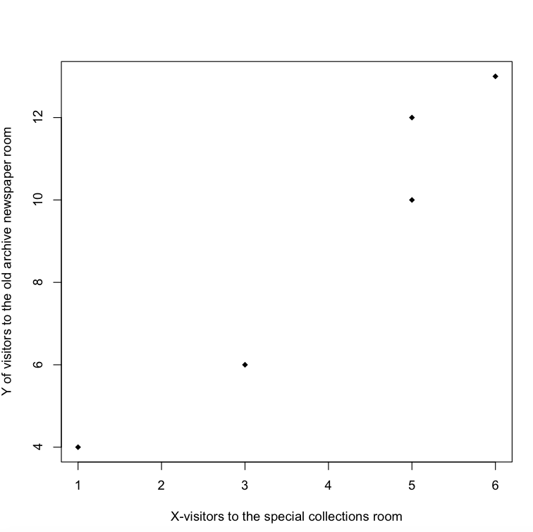
To illustrate our findings, R also provides the ability to create simple plots to illustrate our data.  The code involves creating a plot to better understand our findings:
>plot(x,y, pch=18, xlab=”x-visitors to the special collections room”, ylab=”y of visitors to the old newspaper archive collections room”)

Next, Chapter 7 Probability Theory
Previous, Chapter 5, Descriptive Statistics