
Time series models have been the basis for the study of a behavior or metrics over a period of time. In decisions that involve a factor of uncertainty about the future, time series models have been found to be one of the most effective methods of forecasting. We often encounter different time series models in sales forecasting, weather forecasting, inventory studies, and so on. In the field of information science, Jeong and Kim (2010) reviewed a selected annotated bibliography of core books in order to conduct a time series analysis.
Often the first step in a time series analysis is to plot the data and observe any patterns that might occur over time by using a plot. This helps us to determine whether there appears to be a long-term upward or downward movement or whether the series seems to vary around a horizontal line over time.
The following scenario will show how the plot illustrates the direction of data. In this example, we follow the number of books borrowed from the library from 1982 to 2014 as found in the public library log in New York City. Table 14.1.
| Year | Numbers of books borrowed from the library | |
|---|---|---|
| 1 | 1982 | 1558 |
| 2 | 1984 | 1564 |
| 3 | 1994 | 1407 |
| 4 | 1995 | 1309 |
| 5 | 1986 | 1424 |
| 6 | 1987 | 1321 |
| 7 | 1988 | 1543 |
| 8 | 1989 | 1321 |
| 9 | 1990 | 1488 |
| 10 | 1991 | 1562 |
| 11 | 1992 | 1618 |
| 12 | 1993 | 1686 |
| 13 | 1994 | 1840 |
| 14 | 1995 | 1865 |
| 15 | 1996 | 1636 |
| 16 | 1997 | 1652 |
| 17 | 1998 | 1453 |
| 18 | 1999 | 1698 |
| 19 | 2000 | 1523 |
| 20 | 2001 | 1437 |
| 21 | 2002 | 1387 |
| 22 | 2003 | 1312 |
| 23 | 2004 | 1212 |
| 24 | 2005 | 1201 |
| 25 | 2006 | 1009 |
| 26 | 2007 | 1001 |
| 27 | 2008 | 999 |
| 28 | 2009 | 1764 |
| 29 | 2010 | 1675 |
| 30 | 2011 | 1218 |
| 31 | 2012 | 1212 |
| 32 | 2013 | 1200 |
You will import the file to R by the following command:
>library_borrowing <-read.csv(“C:/Table14.1″, header=T, dec=”,”, sep=”;”)
Note that paths use forward slashes “/” instead of backslashes
>plot(library_borrowing[, 5], type=”1″, lowd=2, col=”red”, xlab=Years”, ylab=”Number of books”, main=”Number of books borrowed from the library” xl)
The result:
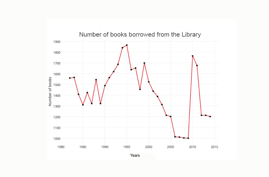
As we can see, this illustration provides an indication and direction of the decline of book borrowing from the library. This trend started in 2000 and stopped in 2009.
The goal of the time series can be classified in five steps:
1. Descriptive: identifying patterns in correlated data—trends and seasonal variations
2. Explanation: understanding and modeling the data
3. Forecasting: prediction of short-term trends from previous patterns
4. Intervention analysis: discovering if a single event changes the time series
5. Quality control: deviations of a specified size indicate a problem
Another aspect of time series is smoothing, a common technique. Smoothing always involves some form of local averaging of data such that the nonsystematic components (variations away from main trend) of individual observations cancel each other out. The most common technique is moving average smoothing, which replaces each element of the series by either the simple or weighted average of n surrounding elements, where n is the width of the smoothing “window.” All of these methods will filter out the noise and convert the data into a smooth curve that is relatively unbiased by outliers.
Among the methods for fitting a straight line to a series of data, Least Square Method is the one used most frequently. The equation of a straight line is Y = a + bx where x is the time period, say year, and Y is the value of the item measured against time, a is the Y intercept, and b is the coefficient of x indicating slope of the trend line. In order to find a and b, the following two equations are calculated:
ΣY = ax + b Σx
ΣXY = a Σx + bΣx2
The code in R:
Based on the library’s example above, we selected the first five numbers:
>time <- c(1986, 1987, 1988, 1989, 1999)
>number <- c(270, 285, 295, 315, 330)
>res=lm(time~number)
>res=lm(time~number)
>res
Coefficients:
(Intercept) 1933.293
Number 0.189
In order to calculate the smoothing of Least Square data, we often use a linear operation. This process converts a single time series {yt} into another time series {xt} by a linear operation. The formula for smoothing using Moving Average:
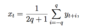
where the analyst chooses the value of q for smoothing. Since averaging is a smoothing process, we can see why the moving average smooths out the noise in a time series. As a result, we will find there exist many variations of the filter described here.
Next, Chapter 15, Visualization Display
Previous, Chapter 13, Analysis of Variances and Chi-Square Test