Computer programs are collections of instructions that tell a computer how to interact with the user, interact with the computer hardware, and process data. In R, the command line interface is what makes R so powerful.

After installing R, you will find the R icon on your desktop. Click on the icon and it will present a window display called R Console.

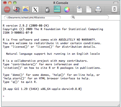
In the last line of the console you will find the prompt, the greater sign or >, which is where you type the code to make R go to work. The convention in this book  is that you will need to type your commands. After you have typed your commands, you will need to press the Return key to see the answer.

So, let’s take a closer look at the syntax of R.
>a <- c(1,2,3,4)
>a
[1] 1 2 3 4
>a + 5
[1] 6 7 8 9

So, what did we do?
The first line: we created a container for “a” that holds the values of 1,2,3,4.
Why do we create a container? In order to capture different data sets or different values (alpha or numeric).
The second line: we ask to display the value of “a”
The third line: displays the result  [1] 1 2 3 4
Note that [1] will always indicate the sum of your calculation.
The fourth line: we add the value of 5 to “a”
The fifth line: displays the result [1] 6, 7, 8, 9.

Like any programming language, R has its own operators. Here are the basic arithmetic operators in R:

Operator	Description
+	addition
–	subtraction
*	multiplication
/	division
^ or **	exponentiation

From our first example, in line 4  we added the value of 5 to “a.” Now, let’s multiply with “a”
>a <- c(1,2,3,4)
>a
[1] 1 2 3 4
>a * 5
[1]  5 10 15 20
This allows us to multiply all the values within “a” without doing it manually.

R Packages
R comes with a standard set of packages, while other packages are available for download and installation, often free of charge. R packages are an easy way to maintain collections of R functions, data sets and compiled code in a well-defined format. According to Friedrich Leisch (2009), the R package can be thought of as equivalent to a scientific article, where the scientific article is the de facto standard to communicate scientific results in a certain format, the same way the R package functions. Using R as the platform allows independent researchers to promote their own packages and lets users adopt any independent packages based on their specific needs.  The R packaging system has been one of the key factors in the overall success of the R project. Packages allow for easy, transparent, and cross-platform extension of the R base system.  There are more than 5000 packages available to download from the open source R CRAN website: https://cran.r-project.org/

In order to install any package, you will type install.packages (the name of the package). For example: install.packages (“lotkalaw”)

This particular package follows Lotka’s Law on author productivity. Lotka’s Law is known for computing author distribution in the scientific community. The package allows the user to measure any data collection by tracing the author productivity. For more information on the package, click here.

More important syntax in R
>search() # search
>q()  # quit
>help ()
>getwd() # print the current working directory – cwd
>ls () # list the objects in the current workspace
>load ( ) # load your dataset into the current session

Vectors 
A vector is the simplest type of data structure in R. Inside the vector are the functions which are self-contained modules of code that can accomplish a specific task.

The following example illustrates the vector function “c” as a function that contains different numeric values:
>c(1, 2, 3)
[1] 1 2 3

Another example that illustrates the vector as a container:
>x <- c(“aa”, “bb”, “cc”, “dd”, “ee”)
[1] aa, bb, cc, dd, ee

The vector index functionality allows us to declare an index inside square brackets [ ]. Here is an example where we are looking for the third value in our vector:
>t <- c(“Bob”, “Richard”, “Colleen”, “Ruth”, “Alex”)
>t[3]
[1] “Colleen”

In Chapter 3, we discussed  different types of variables and their values. In programming, the terminology of variables is a little different. Variables are given names, so that we can assign values to them and refer to them later. Variables typically store values of a given type. In any programming language, we often encounter six types of data:

1. Numeric—holds a decimal value.
For example:
>x <- 1
>x
[1] 1

2. Integers—used to store  “whole” numbers, both positive or negative. To declare an integer variable in R, we use a function called as.integer. We can be confident that x is an integer by applying the as.integer function. For example:
>x = as.integer(-3)
>x
[1]-3 #Note in line two, the sign >x  will print (display) the value of x.
>class(x) # print the class name of x
[1] “integer”

3. Strings—a collection of characters.  A string is a data type integer that presents in the form of text rather than numbers. It comprises a set of characters that can also contain spaces and numbers. For example:
>a <- “hello”
>a
[1] “hello”
>b <- c(“hello”,”3″)
>b
[1] “hello” “3”

4. Characters— represent a single element such as a letter of the alphabet, punctuation or number. In order to convert objects into character values in R, we need to declare this value as a character with the as.character() function:
>x = as.character(0.14)
[1] “0.14”
The strength of the character is when using two characters together.
>firstname = “Alon”; lastname =”Friedman”
>paste(firstname, lastname)
[1] “Alon Friedman”

5. Factor— is an explanatory variable manipulated by the experimenter. In R, factor takes on a limited number of different values; such variables are often referred to as categorical variables. In the textbook, we defined categorical variables which represent types of data that may be divided into groups. To illustrate, the color of hair could be black, white, blond, or grey.  For example:
>a <- c(“blond”, “black”, “white”, “grey”, “blond”, “white”, “white”, “black”)
>a <- factor (c(“blond”, “black”, “white”, “grey”, “blond”, “white”, “white”, “black”))
>a
[1] blond black white grey blond white white black
Levels: black blond grey white

Note, the R factor provides us levels for black blond grey white. A level is the categorization of the data it displays.

6. Logical—under logical variables the values are either True or False. In R the logical value makes a comparison between variables and provides additional functionality by adding/subtracting/etc. For example:
>x = 1; y = 2
>x>y
[1] FALSE

Import data
Data is often kept in spreadsheets, and the most frequently used program is Microsoft Excel. There are several options for importing data from a Microsoft Excel spreadsheet into R. The following four steps are an easy way to import Excel to R:

Step 1—Open the data in Excel and prepare to export it as .csv format.

Step 2—Close the Excel application and create a folder where you will keep this file.

Step 3—Open R and type the setwd command that designates it to be your working directory for R, where you will keep all your files with R.

Step 4—Type the following code:
>read.table function in R to import the data.

To import data where the file name is “first.csv” and its location is in the C drive, type the following code:
>first.cvs <-read.table(“c:/first.csv”, header=T)

Next, Chapter 5, Descriptive Statistics
Previous, Chapter 3, Data (Types and Collection Methods)