
In Chapter 11, we discussed the hypothesis testing methodology, where we illustrated how to draw conclusions about possible differences between the two variables we outlined in our hypothesis (x and y). A critical tool for carrying out the analysis is the analysis of variance (ANOVA). It allows a researcher to differentiate treatment results based on easily computed statistical quantities from the treatment outcome. This chapter will introduce the analysis of variance (ANOVA) and its contribution to analyzing more than two groups at a time.
In an experimental study, various treatments are applied to test subjects and the response data is gathered for analysis. The ANOVA tests uses a null hypothesis where samples in two or more groups are drawn from populations with the same mean values. It enables a researcher to differentiate treatment results. The information obtained from a sample determines the treatment outcome using estimation as the process about a population.
Statisticians use sample statistics to estimate population parameters. For example, sample means are used to estimate population means; sample proportions to estimate population proportions. An estimate of a population parameter may be expressed in two ways:
1. Point estimate. A point estimate of a sample parameter is a single value, a statistic, of a population. For example, the sample mean x is a point estimate of the population mean μ. Similarly, the sample proportion p is a point estimate of the population proportion P.
2. Interval estimate. An interval estimate is defined by two numbers between which a population parameter is said to lie. For example, a < x < b is an interval estimate of the population mean μ. It indicates that the population mean is greater than a but less than b.
One way to find the confidence interval is by conducting a sample. The advantage of the sample in this case is that you don’t know anything about a population’s behavior. You will use the t-distribution to find the confidence interval. The easy way to find the t-distribution is to find the Degree of Freedom. The term Degrees of Freedom, abbreviated as df, has often been defined as how certain we are that our sample population is representative of the entire population.
When calculating Degrees of Freedom, you have three conditions that need to be met regarding the type of variables found in your data.
1) For one independent variable: df = (r-1), where r equals the number of levels of the independent variable
2) For two independent variables: df = (r-1) (s-1), where r and s are the number of levels of the first and second independent variables, respectively.
3) For three independent variables: df = (r-1) (s-1) (t-1), where r, s and t are the number of levels of the first, second and third independent variables, respectively.
The code in R
As discussed in Chapter 9, R comes with a rich set of probability distribution functions, and four consistent ways of accessing them using r, d, q, and p. The r returns randomly generated numbers, d returns the height of the probability density function, q returns the inverse cumulative density function (quantiles) and p returns the cumulative density function. If you combine these with the name of the distribution, in this case norm distribution – rnorm(), dnorm(), qnorm(), and pnorm() – you will get different types of distributions. For example, you can generate random numbers, find the value of the function at a specific point, produce a critical value, and calculate a p-value.
Most distributions require one or more parameters to define the shape of the distribution. The F distribution is a right-skewed distribution used most commonly in Analysis of Variance. When referencing the F distribution, the numerator degrees of freedom are always given first, as switching the order of degrees of freedom changes the distribution (e.g., F(10,12) does not equal F(12,10) ). For the F distribution, you need the degrees of freedom for the numerator (df1) and the denominator (df2). To generate n=50 random numbers, you would type:
>rf(n=50, df1=15, df2=20)
[1] 0.6879144 0.6449737 0.5289995 0.5585555 1.1359455 1.0913042 0.7730051 1.4645508 1.9845975 0.7559698 0.8746356
[12] 0.4501796 2.0243666 1.6722989 1.9648821 0.5972655 1.2176494 1.5123766 0.9724616 2.6671159 0.9443942 1.9013938
[23] 0.5635537 1.5986902 0.8151447 0.6866006 0.4520317 0.9963964 0.3705470 1.0114762 1.2404028 1.1314835 0.7744022
[34] 1.6424297 1.6117785 1.0169789 1.1452108 1.0637519 0.4932719 1.3657477 1.2916658 1.2676952 0.7146134 2.3167524
[45] 0.7880809 1.2984185 0.9003225 1.1734979 0.6619288 1.3323957
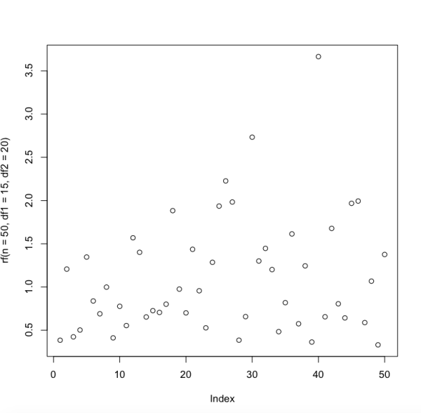
You can also use a histogram to illustrate this type of distribution and see the approximate shape of the F distribution of this case. The code in R:
>plot(rf(n=50, df1=15, df2=20))
Analysis of variance (ANOVA) as discussed above is used to determine whether the mean differences found in sample data are greater than can be reasonably explained by chance alone. ANOVA can be used to evaluate differences between two or more treatments (or populations).
For example, you might have data on student research in the library performance in non-assessed tutorial exercises as well as their final grading. You are interested in how library tutorial performance is related to final grade. ANOVA allows you to break up the group according to the grade and then see if performance is different across these grades.
There are two types of ANOVA testing:
1. One-Way ANOVA
2. Two-Way ANOVA
Under One-Way ANOVA you are looking at the differences between the groups. There is only one grouping (final grade) which you are using to define the groups. This is the simplest version of ANOVA. Two-Way ANOVA allows you to examine the differences between two or more groups.
Here we will illustrate One-Way ANOVA. In order to measure ANOVA, we use our hypothesis in order to evaluate F-value. The F-value has two degrees of freedom: degrees of freedom for the numerator and degrees of freedom for the denominator. The F-value is often used to calculate the sampling distribution derived from the ratio of two sample variances (s2) estimating identical population variances (σ2). Academic journals almost always require researchers to provide the degrees of freedom, the F-value and the p-value but unfortunately, many people (including reviewers) only look at the p-value, overlooking the degrees of freedom.
The code in R:
The d prefix, such as df(), is useful for finding the value of F distribution. In other words, d gives you the height of the probability distribution. In order to run F distribution in R, you need to supply the degrees of freedom for the numerator and the denominator, and in this case you need to specify the value of F for which you want the F function. For an F distribution value of 2.3, with 15 and 20 degrees of freedom, the F function is given by:
>df(x=2.3, df1=15, df2=20)
[1] 0.07871035
Note, this is only one way to calculate F distribution in R. The second option calculating the F value and ANOVA is using data.frame. To generate a data.frame, you combine the two measurements you conducted. In the following example, the value represents measurement and the group represents the value of the groups you measure. The third line is the creation of data.frame of the two variables. In this example, R will provide us the result based on our hypothesis testing. The code in R:
>value <- c(1,1,2,3,1,3,2,4,1,2,6,5,1,3,5,1,2,3,4)
>group <- c(0,0,0,0,0,0,0,0,0,0,1,1,1,1,1,1,1,1,1)
>data <- data.frame(group, value)
>data # will display the two variables
The F-test:
The F-test is designed to test if two population variances are equal to one another. It does that by comparing the ratio of two variances/groups. So, if the variances are equal, the ratio of the variances will be 1. The formula for F-test for a One-Way ANOVA is:
![]()
where  represents the sample mean, the ni is the number of observations in the ith group,
  stands for the overall mean of the data, and K denotes the number of groups.
The F-test Code in R:
>af.test(data[data[“group”]==0,2],
>data[data[‘group’]==1,2]) ### F-test to compare two variances
data: data[data[“group”] == 0, 2] and data[data[“group”]== 1, 2]
F = 0.3419, num df = 9, denom df = 8, p-value = 0.1306
alternative hypothesis: true ratio of variances is not equal to 1
95 percent confidence interval: 0.07846272 1.40237802
sample estimates:
ratio of variances: 0.3418803
The Chi-Square Test
The chi-square test is a statistical test that can be used to determine whether observed frequencies are significantly different from expected frequencies. The chi-square test is used to examine differences with categorical variables. We can estimate how closely an observed distribution matches an expected distribution—we’ll refer to this as the goodness-of-fit test. Or, we can estimate whether two random variables are independent.
The chi-square goodness-of-fit test is a single-sample nonparametric test, also referred to as the one-sample goodness-of-fit test or Pearson’s chi-square goodness-of-fit test. It is used to determine whether the distribution of cases (e.g., participants) in a single categorical variable (e.g., “gender,” traditionally consisting of two groups “male” and “female”) follows a known or hypothesized distribution (e.g., a distribution that is “known,” such as the proportion of males and females in a country; or a distribution that is “hypothesized,” such as the proportion of males versus females that we anticipate voting for a particular political party in the next elections). The proportion of cases expected in each group of the categorical variable can be equal or unequal (e.g., we may anticipate an “equal” proportion of males and females reading books about baking, or an “unequal” proportion, with 70% of those books’ readers being male and only 30% female).
Example:
For illustration purposes: we use the study published by Cherry and Duff (2002), titled: “Studying digital library users over time: a follow-up survey of Early Canadiana Online.” The article was published in Information Research, Vol. 7 No. 2, January 2002. Note: we revised the numbers to make this question easier to understand and calculate.
The study gave the following information on the age distribution of library online users using Early Canadiana. 35% are between 18 and 34 years old, 51% are between 35 and 64 years old and 14% are 65 year old or older. Our revised data provide us the following library habits. The following table is not consistent with the values given in the article.
| Age of library users | Frequency |
| 18-34 | 36 |
| 35-64 | 130 |
| 65 and over | 34 |
Suppose that the data resulted from a random sample of 200 Canadian library users. Based on these sample data, can we conclude that one or more of the three age groups use Early Canadiana?
The code in R:
Note: we created two variables Age and Frequency of use. Under the Age group we count the average age.
>age <-c(18, 29, 35)
>frequency <-c(36,130, 34)
>chisq.test(age,frequency)
Pearson’s chi-squared test data: age and frequency
x-squared = 6, df = 4, p-value = 0.1991
R Warning message:
In chisq.test(age, frequency): Chi-squared approximation may be incorrect
R provides a warning message regarding the frequency of measurement outcome that might be a concern.
In order to answer our question whether the three age groups use Early Canadiana we will use the p-value. In Chapter 11, we discussed the p-value with regard to hypothesis testing. We stated that if p-value is smaller than α, we can reject H0. In this example, we did not state our hypothesis and if we did, we would accept or reject our hypothesis based on the value of the H0 and value of p-value. In this case the p-value is equal to 0.1991.
Next, Chapter 14, Time Series and Predictive Analysis
Previous Chapter, Chapter 12, Correlation and Regression